Reinforcement Learning: Q and Q(λ) speed difference on Windy Grid World environment

Question

Preface:

I have attempted to solve this Windy-Grid-World env. Having implemented both Q and Q(λ) algorithm, the results are pretty much the same (I am looking at steps per episode).

Problem:

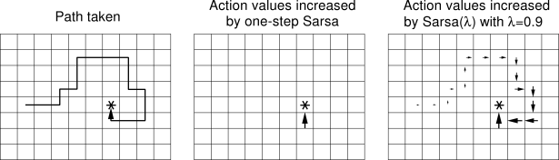
From what I have read, I believe that a higher lambda parameter should update more states further back leading up to it; therefore, the amount of steps should decrease much more dramatically than regular Q-learning. This image shows what I am talking about.

Is this normal for this environment or have I implemented it wrong?

Code:

import matplotlib.pyplot as plt
import numpy as np
from lib.envs.windy_gridworld import WindyGridworldEnv
from collections import defaultdict

env = WindyGridworldEnv()


def epsilon_greedy_policy(Q, state, nA, epsilon):
    '''
    Create a policy in which epsilon dictates how likely it will 
    take a random action.

    :param Q: links state -> action value (dictionary)
    :param state: state character is in (int)
    :param nA: number of actions (int)
    :param epsilon: chance it will take a random move (float)
    :return: probability of each action to be taken (list)
    '''
    probs = np.ones(nA) * epsilon / nA
    best_action = np.argmax(Q[state])
    probs[best_action] += 1.0 - epsilon

    return probs

def Q_learning_lambda(episodes, learning_rate, discount, epsilon, _lambda):
    '''
    Learns to solve the environment using Q(λ)

    :param episodes: Number of episodes to run (int)
    :param learning_rate: How fast it will converge to a point (float [0, 1])
    :param discount: How much future events lose their value (float [0, 1])
    :param epsilon: chance a random move is selected (float [0, 1])
    :param _lambda: How much credit to give states leading up to reward (float [0, 1])

    :return: x,y points to graph
    '''

    # Link state to action values
    Q = defaultdict(lambda: np.zeros(env.action_space.n))
    # Eligibility trace
    e = defaultdict(lambda: np.zeros(env.action_space.n))

    # Points to plot
    # number of episodes
    x = np.arange(episodes)
    # number of steps
    y = np.zeros(episodes)

    for episode in range(episodes):
        state = env.reset()

        # Select action
        probs = epsilon_greedy_policy(Q, state, env.action_space.n, epsilon)
        action = np.random.choice(len(probs), p=probs)

        for step in range(10000):

            # Take action
            next_state, reward, done, _ = env.step(action)

            # Select next action
            probs = epsilon_greedy_policy(Q, next_state, env.action_space.n, epsilon)
            next_action = np.random.choice(len(probs), p=probs)

            # Get update value
            best_next_action = np.argmax(Q[next_state])
            td_target = reward + discount * Q[next_state][best_next_action]
            td_error = td_target - Q[state][action]

            e[state][action] += 1

            # Update all states
            for s in Q:
                for a in range(len(Q[s])):

                    # Update Q value based on eligibility trace
                    Q[s][a] += learning_rate * td_error * e[s][a]

                    # Decay eligibility trace if best action is taken
                    if next_action is best_next_action:
                        e[s][a] = discount * _lambda * e[s][a]
                    # Reset eligibility trace if random action taken
                    else:
                        e[s][a] = 0

            if done:
                y[episode] = step
                e.clear()
                break

            # Update action and state
            action = next_action
            state = next_state

    return x, y

You can check out my Jupyter Notebook here if you would like to see the whole thing.

Answer 1

There is no problem with your implementations.

What you have implemented for Q(λ) is the Watkins' version of Q(λ). In his version, the eligibility traces will be zero out for non-greedy actions, and only backed up for greedy actions. As mentioned in eligibility traces (p25), the disadvantage of Watkins' Q(λ) is that in early learning, the eligibility trace will be “cut” (zeroed out) frequently, resulting in little advantage to traces. Maybe that's the reason why your Q-learning and Q(λ)-learning have very similar performance.

You can try other eligibility traces, such as Peng's eligibility or Naive eligibility, to check whether there are any boosts in performances.